amibroker

HomeKnowledge Base

Points-only backtest

Some users coming from Metastock ask for “points-only” test.

One needs to know that AmiBroker features way more sophisticated futures mode than MS ever had: http://www.amibroker.com/guide/h_futbacktest.html
It provides full support for futures trading, handling margin deposit, point value, etc.

“Points-only” test is kind of the simplest possible case, but if you want to do just that, it can be implemented using these two lines:

SetOption("FuturesMode"True );
SetPostionSize1spsShares ); // trade just 1 contrac

That is all what you need to add to your formula to get point-only test.

About floating point arithmetic

In general, to represent numbers with fractional parts, computers use a “floating point” binary representation. Floating point arithmetic is also used by AmiBroker for AFL calculations. For some more information about floating point representation in general see the following article, here we will only discuss some practical aspects.

http://en.wikipedia.org/wiki/Floating_point

Floating point calculations are performed in hardware by FPU (Floating Point Unit), which today is a part of your computer’s processor (CPU). The calculations are performed according to IEEE754 standard (see below) that all CPU manufacturers follow.

Internally in computers all numbers are represented in binary system.
This fact has some important consequences in practice. One of it is that some fractions that have finite representation in decimal system are not finite in binary.

For example, 0.1 is endless (infinite) fraction in binary system, as 1/3 or 2/3 fractions are in decimal system.

The mantissa of 0.1 fraction in binary system is cyclical:
1001 1001 1001 1001 1001 1001 1001 1001 1001 1001 1001 1001 1001 1001 1001 1001 1001 (1001)* …….

* represents endless cycle.

Since computers operate on limited word length, 32 bit binary representation of 0.1 is:
01111011 10011001100110011001100 (not rounded) (in decimal it is 0.09999999403953552)
or
01111011 10011001100110011001101 (rounded) (in decimal it is 0.10000000149011612)

Later is used by FPU (floating point processor) in your CPU because it has smaller relative error. If you add it nine times you will end up with 0.9000000134110449 which is of course higher than 0.9.

It will be easier for you to understand when explaining on decimal numbers. For example 2/3 represented in decimal is:
0.666666667

Now add THREE times this number (0.666666667 + 0.666666667 + 0.666666667) and what you will get?
2.000000001 and that is greater than 2.

Therefore, it is rule in programming, NEVER use fractions for loop counters. For that reason you should not use fractions in Optimize(), or if you need to use them use them in WISE way by adding HALF of “step” value to the “max” value.

step 0.1;
Optimize("x"0.50.10.9 step/2step)

Another thing to keep in mind is that 32-bit floating point number has only 7 significant digits (those digits that carry meaning contributing to its precision). So in 123.4567 all digits are significant and accurate, but in 123.456789, last two digits (‘8’ and ‘9’) are not significant and subject to floating point rounding – see links below).

See also:
About significant figures:
http://en.wikipedia.org/wiki/Significant_figures

IEEE754 conversion calculators:
http://babbage.cs.qc.edu/IEEE-754/Decimal.html
http://babbage.cs.qc.edu/IEEE-754/32bit.html

IEEE754 standard description:
http://en.wikipedia.org/wiki/IEEE_754-1985

Essay about comparing floatin point numbers:
http://www.cygnus-software.com/papers/comparingfloats/comparingfloats.htm

Microsoft Knowledge Base: “Precision and Accuracy in Floating-Point Calculations”
http://support.microsoft.com/kb/125056

Using 32-bit floating point (as opposed to 64-bit double precision) has two main advantages:
a) consumes HALF of memory required for doubles (this *is* important, more important that you think, because if you have for example an array of 500000 elements, in floats it is 2MB and it fits into CPU cache, while in doubles it would be 4MB and may not fit into CPU cache).
b) 32-bit floating point numbers can be computed much faster. It simply takes less processor cycles to compute 32-bit float than 64-bit float. 64-bit version of AmiBroker is going even further and is using SSE2 instructions. This means that vectors of 4 single-precision numbers are processed in parallel using single SSE2 instruction on SINGLE processor. This gives more speed on single core than achievable using multiple cores.

Note also AmiBroker does use double precision (64bit/SSE2) or extended precision (80bit/x87) where it is necessary (for certain internal calculations).

Note also that due to the architectural differences between compilers for 32-bit and 64-bit programs,
small numerical differences may exist between 32-bit and 64-bit version of AmiBroker due to the fact that 32-bit version uses x87 FPU code while 64-bit version uses SSE2 code and the underlying floating point hardware is different and operate slightly differently.
x87 FPU code internally offers more (80bit) precision than SSE2 (64-bit).
For in-depth discussion see:
https://randomascii.wordpress.com/2012/03/21/intermediate-floating-point-precision/

Study() function in logarithmic scale

IMPORTANT: This article applies ONLY to AmiBroker version 5.24 and earlier. Version 5.25 includes native support for log scale in Study() function and this workaround is no longer needed.

Some of you may have tried using Study() function in logarithmic scale charts and noticed that the output of Study() function becomes curved line (not straight) as soon as logarithmic scale is used.

Before giving you solution, I would like to state some obvious things:
A straight line in log scale is NOT straight line in linear scale and vice versa. Trendlines drawn in log scale do NOT cross at the same points (except beginning and ending) as same trendline drawn in linear scale. This is pretty much the same in all charting programs.

As for the Study() function – it always uses LINEAR equation y = a*x + b regardless of particular chart scale. So, Study() always produces straight line in the linear price domain, so “a” coefficient is constant and represents the slope in price terms (dollar per bar)

This is done so, because Automatic Analysis does not have a concept of “scale” (linear vs logarithmic), therefore if Study() function was dependent on given pane setting it would not produce the same result, if the same formula was used in automatic analysis.

If you want to have “straight” line in the logarithmic price domain you need to convert to log domain in the formula, as shown in the code below


function StudyInLogScaleStudyidChartid )
{
  if( 
Version() < 5.25 )
  {
   
SetBarsRequiredsbrAllsbrAll );

   
temp StudyStudyidChartid );

   
bi BarIndex();

   
beg LastValueValueWhenExRemtemp), bi ) ); 
   
end LastValueValueWhentempbi ) );

   
result Null;
 
   if( 
beg BarCount AND end BarCount )
   {
    
begval tempbeg ];
    
endval tempend ];
    
factor endval/begval;

    for( 
beg<= endi++ )
    {
      
result] = begval factor ^ ( ( beg )/( end beg ) ); 
    }
   }
  }
  else
  {
    
result StudyStudyidChartid );
  }

  return 
result;        
}

logscale ParamToggle("Log Scale""Off|On");

SetChartOptionsIIflogScale2), chartLogarithmic );

PlotC"Price"colorBlackstyleCandle );

if( 
logscale AND Version() <= 5.24 )
{
 
ss StudyInLogScale("RE"GetChartID() );
}
else
{
 
ss Study("RE"GetChartID() );
}

Plotss"Study"colorRed )

How to convert from bar-value to pixel co-ordinates

NOTE: This article describes old method of using bar/value coordinates. New code should use GfxSetCoordsMode which allows you to use bar/value without any extra calculations.

Sometimes when using low-level graphics functions it is needed to convert from bar number to pixel X co-ordinate and from price level to pixel Y co-ordinate. Converting between them needs knowing visible bar range, Y-axis value range and pixel dimensions of drawing area. Once these params are known it is just a matter of performing simple scale transformation. The code example below shows how to do that.

function GetVisibleBarCount()
{
 
lvb Status("lastvisiblebar");
 
fvb Status("firstvisiblebar"); 

 return 
MinLvb fvbBarCount fvb );


function 
GfxConvertBarToPixelXbar )
{
 
lvb Status("lastvisiblebar");
 
fvb Status("firstvisiblebar");
 
pxchartleft Status("pxchartleft");
 
pxchartwidth Status("pxchartwidth"); 

 return 
pxchartleft bar  pxchartwidth / ( Lvb fvb );


function 
GfxConvertValueToPixelYValue )
{
 
local MinyMaxypxchartbottompxchartheight

 
Miny Status("axisminy");
 
Maxy Status("axismaxy"); 

 
pxchartbottom Status("pxchartbottom");
 
pxchartheight Status("pxchartheight"); 

 return 
pxchartbottom floor0.5 + ( Value Miny ) * pxchartheight/ ( Maxy Miny ) );


Plot(C"Price"colorBlackstyleHistogram ); 

GfxSetOverlayMode(0);
GfxSelectSolidBrushcolorRed );
GfxSelectPencolorRed ); 

AllVisibleBars GetVisibleBarCount();
fvb Status("firstvisiblebar"); 

for( 
0AllVisibleBars i++ ) 

  
GfxConvertBarToPixelX); 
  
GfxConvertValueToPixelYCfvb ] ); 

  
GfxRectanglex-1y-12y+); 


RequestTimedRefresh(1); // ensure 1 sec refres

Note that when chart scale changes, it will usually require one extra refresh to get low-level graphics alignment to new scale. That’s why we added RequestTimedRefresh call at the end.

AFL execution speed

NOTE: Benchmarks and timings given below are little outdated because article was written back in 2008. Today’s CPUs are faster and memory bandwidth is also higher.

AmiBroker Formula Language (AFL) thanks to its array processing model is able to run at the same speed as code written in assembler (i.e. machine code). The following article explains how.

AFL runs with native assembly speed when using array operations.
A simple array multiplication like this:

Close  H// array multiplication (each array element is multiplied

gets compiled by AmiBroker to just 8 assembly instructions:

loop:
mov edx,dword ptr [esp+58h]
inc esi ; increase counters
add eax,4
cmp esi,edi
fld dword ptr [edx+esi*4-4] ; get element of close array
fmul dword ptr [eax+ecx-4] ; multiply by element of high array
fstp dword ptr [eax-4] ; store result
jl loop ; continue until all elements are processed

As you can see there are three 4 byte memory accesses per loop iteration (2 reads each 4 bytes long and 1 write 4 byte long)

With such tight loop, single processor core running an AFL formula is able to saturate memory bandwidth in majority of most common operations/functions if total array sizes used in given formula exceedes DATA cache size.

On my (2 year old) 2GHz Athlon x2 64 single iteration of this loop takes 6 nanoseconds (see benchmark code below). 6 nanoseconds to process one bar of data, or 166 million bars per second. So, during 6 nanoseconds we have 8 byte reads and 4 byte store. Thats (8/(6e-9)) bytes per second = 1333 MB per second read and 667 MB per second write simultaneously i.e. 2GB/sec combined !

Now if you look at memory benchmarks you will see that 2GB/s is the limit of system memory speed on Athlon x64 (DDR2 dual channel)
And that’s considering the fact that Athlon has superior-to-intel on-die integrated memory controller (hypertransfer)

// benchmark code
// for accurrate results run it on LARGE arrays -
// intraday database, 1-minute interval, 50K bars or more)
GetPerformanceCounter(1);
for(
01000k++ )  H
"Time per single iteration [s]="+1e-3*GetPerformanceCounter()/(1000*BarCount); 

Only really complex operations that use *lots* of FPU (floating point) cycles such as trigonometric (sin/cos/tan) functions are slow enough for the memory to keep up.

QuickAFL facts

QuickAFL(tm) is a feature that allows faster AFL calculation under certain conditions. Initially (since 2003) it was available for indicators only, as of version 5.14+ it is available in Automatic Analysis too.

Initially the idea was to allow faster chart redraws through calculating AFL formula only for that part which is visible on the chart. In a similar manner, automatic analysis window can use subset of available quotations to calculate AFL, if selected “range” parameter is less than “All quotations”.

So, in short QuickAFL works so it calculates only part of the array that is currently visible (indicator) or within selected range (Automatic Analysis).

Your formulas, under QuickAFL, may or may NOT use all data bars available, but only visible (or “in-range”) bars (plus some extra to ensure calculation of used indicators), so when you are using Close[ 0 ] it represents not first bar in entire data set but first bar in array currently used (which is just a bit longer than visible, or ‘in-range’ area).

The QuickAFL is designed to be transparent, i.e. do not require any changes to the formulas you are using. To achieve this goal, AmiBroker in the first execution of given formula “learns” how many bars are really needed to calculate it correctly.

To find out the number of bars required to calculate formula AmiBroker internally uses two variables ‘backward ref’ and ‘forward ref’.

‘backward ref’ describes how many PREVIOUS bars are needed to calculate the value for today, and ‘forward ref’ tells how many FUTURE bars are needed to calculate value for today.

If these numbers are known, during execution of given formula AmiBroker takes FIRST visible (or in-range) bar and subtracts ‘backward ref” and takes LAST visible (or in-range) bar and adds ‘forward ref’ to calculate first and last bar needed for calculation of the formula.

Now, how does AmiBroker know a correct “backward ref” and “forward ref” for the entire formula?
Well, every AmiBroker’s built-in function is written so that it knows its own requirements and adds them to global “backward ref” and “forward ref” each time given function is called from your formula.

The whole process starts with setting initial BackwardRef to 30 and ForwardRef to zero. These initial values are used to give “safety margin” for simple loops/scripts.

Next, when parser scans the formula like this:

Buy Ref MAC40 ), -)

it analyses it and “sees” the MA with parameter 40. It knows that simple moving average of period 40 requires 40 past bars and zero future bars to calculate correctly so it does the following (all internally):

BackwardRef BackwardRef 40;
ForwardRef ForwardRef 0

So now, the value of BackwardRef will be 70 (40+30(initial)), and ForwardRef will be zero.

Next the parser sees Ref( .., -1 );

It knows that Ref with shift of -1 requires 1 past bar and zero future bars so it “accumulates” requirements this way:

BackwardRef BackwardRef 1;
ForwardRef ForwardRef 0

So it ends up with:

BackwardRef 71;
ForwardRef 0

The BackwardRef and ForwardRef numbers are displayed by AFL Editor’s Tools->Check and Profile as well as on charts when “Display chart timing” is selected in the preferences.

If you use Check and Profile tool, it will tell you that the formula

Buy Ref MAC40 ), -)

requires 71 past bars and 0 future bars.

You can modify it to

Buy Ref MAC50 ), -)

and it will tell you that it requires 82 past bars (30+50+2) and zero future bars.

If you modify it to

Buy Ref MAC50 ), )

It will tell you that it needs 80 past bars (30+50) and ONE future bar (from Ref).

Thanks to that your formula will use 80 bars prior to first visible (or in-range) bar leading to correct calculation result, while improving the speed of execution by not using bars preceding required ones.

IMPORTANT NOTES

It is very important to understand, that the above estimate requirements while fairly conservative,
and working fine in majority of cases, may NOT give you identical results with QuickAFL enabled, if your formulas use:
a) JScript/VBScript scripting
b) for/while/do loops using more than 30 past bars
c) any functions from external indicator DLLs
d) certain functions that use recursive calculation such as very long exponential averages or TimeFrame functions with much higher intervals than base interval

In these cases, you may need to use SetBarsRequired() function to set initial requirements to value higher than default 30. For example, by placing

SetBarsRequired1000)

at the TOP of your formula you are telling AmiBroker to add 1000 bars PRIOR to first visible (or in-range) bar to ensure more data to stabilise indicators.

You can also effectively turn OFF QuickAFL by adding:

SetBarsRequiredsbrAllsbrAll )

at the top of your formula. It tells AmiBroker to use ALL bars all the time.

It is also worth noting that certain functions like cumulative sum (Cum()) by default request ALL past bars to guarantee the same results when QuickAFL is enabled. But when using such a function, you may or may NOT want to use all bars. So SetBarsRequired() gives you also ability to DECREASE the requirements of formula. This is done by placing SetBarsRequired at the END of your formula, as any call to SetBarsRequired effectively overwrites previously calculated estimate. So
if you write

Cum);
SetBarsRequired1000); // use 1000 past bars DESPITE using Cum(

You may force AmiBroker to use only 1000 bars prior first visible even though Cum() by itself would require all bars.

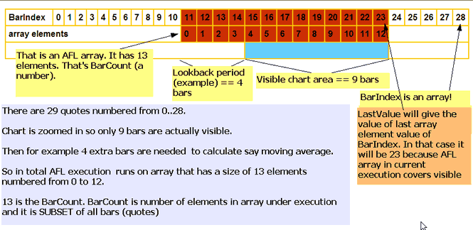
It is also worth noting that when QuickAFL is used, BarIndex() function does NOT represent elements of the AFL array, but rather the indexes of ENTIRE quotation array. With QuickAFL turned on, an AFL array is usually shorter than quotation array, as illustrated in this picture:

QuickAFL, BarIndex and BarCount

SPECIAL CASE: AddToComposite function

Since AddToComposite creates artificial stock data it is desirable that it works the same regardless of how many ‘visible’ bars there are or how many bars are needed by other parts of the formula.

For this reason internally AddToComposite does this:

SetBarsRequiredsbrAllsbrAll )

which effectivelly means “use all available bars” for the formula. AddToComposite function simply tells the AFL engine to use all available bars (from the very first to the very last) regardless of how formula looks like. This is to ensure that AddToComposite updates ALL bars of the composite

The side-effect is that “Check And Profile” feature will see that it needs to reference future bars and display a warning even though this is false alert because AddToComposite itself has no impact on trading system at all.

Now why this shows only when flag atcFlagEnableInBacktest is on ??
It is simple: this is so because it means that AddToComposite is ACTIVE in BACKTEST.
http://www.amibroker.com/guide/afl/afl_view.php?name=ADDTOCOMPOSITE

Since “Check And Profile” uses “BACKTEST” state you get such result.

If atcFlagEnableInBacktest is not specified AddToComposite is not enabled in Backtest and hence does not affect calculation of BackwardRef and ForwardRef during “Check And Profile”.

BACKWARD COMPATIBILITY NOTES

a) QuickAFL is available in Automatic Analysis in version 5.14.0 or higher
b) sbrAll constant is available in Automatic Analysis in version 5.14.0 or higher. If you are using older versions you should use numeric constant of: 1000000 instead.

Historical portfolio backtest metrics

Recently on the AmiBroker mailing list some users expressed wish to have access to some of portfolio backtest metrics available in “historical” form (i.e. as date series, as opposed to scalars), so they can be plotted as an indicator.

Implementing such functionality is actually easy with existing tools and does not require any OLE scripts. Everything you need is small custom-backtester procedure that just reads built-in stats every bar and puts them into composite ticker.
In the accompanying indicator code all you need to do is simply use Foreign() function to access the historical metrics data generated during backtest.

The code below shows the BACKTEST formula with custom backtester part:

// Replace lines below with YOUR TRADING SYSTEM
EnableRotationalTrading();
PositionScore 1/RSI(14);
PositionSize = -25;
SetOption("WorstRankHeld");
SetOption("MaxOpenPositions"); 

////////////////////////////////////////
// BELOW IS ACTUAL CUSTOM BACKTESTER PART
// that can read any built-in metric (in this example UlcerIndex)
// and store it into composite ticker for further
// retrieval as data series

SetOption("UseCustomBacktestProc"True ); 

if( 
Status("action") == actionPortfolio )
{
  
bo GetBacktesterObject();

  
bo.PreProcess(); // Initialize backtester

  // initialize with null
  // you can have as many historical metrics as you want
  // (just duplicate line below for many metrics you want)
  
MyHistStat1 Null;
  
MyHistStat2 Null// add your own 

  
for(bar=0bar BarCountbar++)
  {
   
bo.ProcessTradeSignalsbar );
  
   
// recalculate built-in stats on EACH BAR
   
stats bo.GetPerformanceStats); 
 
   
// the line below reads the metric and stores it as array element
   // you can add many lines for each metric of your choice
   
MyHistStat1bar ] = stats.GetValue("UlcerIndex"); // get ulcer index value calculated this bar
   
MyHistStat2bar ] = stats.GetValue("WinnersPercent"); // add your own

  
}

  
bo.PostProcess(); // Finalize backtester

  // now STORE the historical data series representing the metric of your choice
  // duplicate the line below for as many metrics as you want
  
AddToCompositeMyHistStat1"~~~UI_HISTORICAL""X"atcFlagEnableInPortfolio atcFlagDefaults );

  
// you can add your own as shown below
  
AddToCompositeMyHistStat2"~~~WP_HISTORICAL""X"atcFlagEnableInPortfolio atcFlagDefaults ); 

In the code above, for illustration purposes, we are exporting UlcerIndex and Winners Percent metrics as data series. They are stored in composite tickers for easy retrieval from indicator level.
You can easily extend code to include ANY number of metrics you want.

Now in order to Plot metrics as indicators, use this simple formula:

PlotForeign("~~~UI_HISTORICAL""UlcerIndex Historical"colorRedstyleLine );
PlotForeign("~~~WP_HISTORICAL""Winners Percent"colorBluestyleLine styleOwnScale )

As you can see with one Foreign function call you can read the historical value of any metric generated by the backtester.

NOTE: when running backtest please setup a filter in AA that EXCLUDES composites (group 253) from backtest set.

Big symbol text in the background

Recently I heard the suggestion to add a security symbol written in big letters in the chart background. Well, actually it is pretty simple to do using low-level gfx. Just add this code sniplet anywhere in your chart formula.

GfxSetOverlayMode(1);
GfxSelectFont("Tahoma"Status("pxheight")/);
GfxSetTextAlign);// center alignment
GfxSetTextColorColorRGB200200200 ) );
GfxSetBkMode(1); // transparent
GfxTextOutName(), Status("pxwidth")/2Status("pxheight")/12 )

UPDATE: I have added transparent mode, so it works fine on non-white backgrounds too.

Getting started with automatic Walk-Forward optimization

Recently released AmiBroker 5.05 BETA features the automatic Walk-Forward Optimization mode.

The automatic Walk forward optimization is a system design and validation technique in which you optimize the parameter values on a past segment of market data (“in-sample”), then test the system forward in time on data following the optimization segment (“out-of-sample”). You evaluate the system based on how well it performs on the test data (“out-of-sample”), not the data it was optimized on.

To use Walk-Forward optimization please follow these steps:

  1. Goto Tools->Automatic Analysis
  2. Click Settings button, then switch to “Walk-Forward tab”
  3. Here you can see Walk forward settings for In-sample optimization, out-of-sample backtest
    “Start” and “End” dates mark initial period begin / end
    This period will be moved forward by “Step” until the “End” reaches the “Last” date.
    The “Start” date can move forward by “step” too, or can be anchored (constant) if “Anchored” check is on.
    If you mark “Use today” then “Last” date entered will be ignored and TODAY (current date) will be used instead

    By default an “EASY MODE” is selected which simplifies the process of setting up WF parameters.
    It assumes that:
    a) Out-of-sample segment immediatelly follows in-sample segment
    b) the length of out-of-sample segment equals to the walk-forward step

    Based on these two assumptions the “EASY” mode takes in-sample END date and sets
    out-of-sample START date to the following day. Then adds in-sample STEP and this becomes out-of-sample END date.
    In-sample and Out-of-sample step values are set to the same values.

    The “EASY” mode guarantees correctness of WF procedure settings.

    In the “ADVANCED” mode, the user has complete control over all values, to the extent that
    they may not constitute valid WF procedure.
    The interface allows to selectivelly disable in-sample and out-of-sample phases using checkboxes at top
    (for special things like runnign sequential backtests without optimization).

    All settings are immediatelly reflected in the PREVIEW list that shows all generated IS/OOS segments and their dates.

    The “Optimization target” field defines the optimization raport COLUMN NAME that
    will be used for sorting results and finding the BEST one. Any built-in column can be used
    (as appears in the optimization output), or you can use any custom metric that you define
    in custom backtester. The default is CAR/MDD, you can however select any other built-in metric from the combo.
    You can also TYPE-IN any custom metric that you have added via custom backtester interface.

  4. Once you defined Walk-Forward settings, please go to Automatic Analysis and
  5. press the dropdown ARROW on the Optimize button and select “Walk Forward Optimization”

This will run sequence of optimizaitons and backtest and the results will be displayed in the “Walk Forward” document that is open in the main application frame.
When optimization is running you can click “MINIMIZE” button on the Progress dialog to minimize it – this allows to see the Walk Forward output during the optimization steps.

IN-SAMPLE and OUT-OF-SAMPLE combined equity

Combined in-sample and out-sample equities are available by
~~~ISEQUITY and ~~~OSEQUITY composite tickers (consecutive periods of IS and OOS are concatenated and scaled to
maintain continuity of equity line – this approach assumes that you generally speaking are compounding profits)
To display IS and OOS equity you may use for example this:

PlotForeign("~~~ISEQUITY","In-Sample Equity"colorRedstyleLine);
PlotForeign("~~~OSEQUITY","Out-Of-Sample Equity"colorGreenstyleLine);
Title "{{NAME}} - {{INTERVAL}} {{DATE}} {{VALUES}}"

Low-level gfx example: Yearly/monthly profit chart

The code below is an little bit more complex example of Low Level Graphics functions (see http://www.amibroker.com/guide/a_lowlevelgfx.html)

It allows to display three kinds of charts:

  1. yearly/monthly profit table
  2. yearly profit bar chart
  3. average monthly profit bar chart

The type of chart is switchable from Parameters dialog.

It should be applied to ~~~EQUITY – portfolio equity symbol (so it only produces output if you run backtest before using it).


SetBarsRequired(1000000,1000000);
eq Foreign("~~~EQUITY""C" );

yr Year();
mo Month();

YearChange yr != Refyr, -);
MonChange mo != Refmo, -);

FirstYr 0;
LastYr 0;

startbar 0;

////////////////////////////
// SKIP non-trading bars
////////////////////////////
for( 0BarCounti++ )
{
  if( 
eq] )
  {
    
startbar i;
    break;
  } 
}

////////////////////////////
// collect yearly / monthly changes in equity
// into dynamic variables
////////////////////////////

LastYrValue eqstartbar  ];
LastMoValue eqstartbar  ];

MaxYrProfit MinYrProfit 0;
MaxMoProfit MinMoProfit 0;

for( 
startbar 1BarCounti++ )
{
  if( 
YearChange] || == BarCount )
  {
    
Chg 100 * ( -eq] / LastYrValue );
    
VarSet("ChgYear"yr], Chg );

    
MaxYrProfit MaxMaxYrProfitChg );
    
MinYrProfit MinMinYrProfitChg );

    if( 
FirstYr == FirstYr yr];
    
LastYr yr];

    
LastYrValue eq];
  }

  if( 
MonChange ] || == BarCount )
  {
    
mon mo];

    
Chg 100 * ( -eq] / LastMoValue );

    
VarSet("ChgMon" yr] + "-" monChg );
    
VarSet("SumChgMon"monChg NzVarGet("SumChgMon"mon ) ) );
    
VarSet("SumMon" monNzVarGet("SumMon"mon ) ) );
 
    
MaxMoProfit MaxMaxMoProfitChg );
    
MinMoProfit MinMinMoProfitChg );

    
LastMoValue eq];
  }
}

/////////////////////////////////////////////////
// Drawing code & helper functions
////////////////////////////////////////////////

GfxSetOverlayMode);

CellHeight = (Status("pxheight")-1)/(LastYr FirstYr ); 
CellWidth = (Status("pxwidth")-1)/14
GfxSelectFont"Tahoma"8.5 ); 

GfxSetBkMode);

function 
PrintInCellstringrowCol 
{
 
Color =  ColorRGBIIfrow == || col == || col == 13220255 ), 255IIfrow 2255220 ) );
 
GfxSelectSolidBrushColor   );
 
GfxRectangleCol CellWidth
                    
row CellHeight, (Col ) * CellWidth 1
                    (
row ) * CellHeight  1); 
 
GfxDrawTextstringCol CellWidth 1
                    
row CellHeight 1
                    (
Col ) * CellWidth, (row ) * CellHeight32+); 


YOffset 25;
XOffset 15;

function 
DrawBartextbarnumbarsyMinyMaxy )
{
 
BarWidth = (Status("pxwidth") - XOffset )/( numbars ); 
 
BarHeight Status("pxheight") - YOffset;
 
relpos = ( Miny ) / (Maxy Miny );

 
xp XOffset + ( bar 0.5 ) * BarWidth;
 
yp YOffset BarHeight * ( relpos );
 
xe XOffset + ( bar ) * BarWidth;
 
ye YOffset BarHeight * ( - ( -miny )/( maxy miny ) );
  
 if( 
)
 {
 
GfxGradientRectxpyp,
                  
xe ye,
                  
ColorHSB70255 relpos255 ), ColorHSB7020255 ) );
 }
 else
 {
 
GfxGradientRectxpye,
                  
xe yp,
                  
ColorHSB020255 ), ColorHSB0255 * ( relpos ), 255 ) );
 }
 
GfxTextOuttextxpye );
 
GfxTextOutStrFormat("%.2f"), xpyp );
}    

function 
DrawLevelsMinyMaxy )
{
  
range Maxy Miny;

  
grid 100;
  if( 
range 10 grid 1;
  else 
  if( 
range 20 grid 2;
  else 
  if( 
range 50 grid 5;
  else 
  if( 
range 100 grid 10;
  else 
  if( 
range 200 grid 20;
  else 
  if( 
range 500 grid 50;

  
_TRACE("grid = "+grid +" range "+range );
  
  
width Status("pxwidth") - XOffset;
  
height Status("pxheight") - YOffset;

  
GfxSelectPencolorBlack1);
  for( 
grid ceilMiny grid ); <= grid floorMaxy grid ); += grid )
  {
    
yp =  YOffset Height * ( -  ( Miny ) / (Maxy Miny ) );

    
GfxMoveToXOffsetyp );
    
GfxLineToXOffset width yp );
    
GfxTextOut""yXOffset widthyp );
  }

  
GfxSelectPencolorBlack1);
  
GfxMoveToXOffsetYOffset );
  
GfxLineToXOffset widthYOffset );
  
GfxLineToXOffset widthYOffset Height );
  
GfxLineToXOffset YOffset Height );
  
GfxLineToXOffset YOffset );
}

MonthNames "Jan,Feb,Mar,Apr,May,Jun,Jul,Aug,Sep,Oct,Nov,Dec";

function 
DisplayProfitTable( )
{
 
Header "Year,"+MonthNames+",Yr Profit%";
 for( 
Col 0; (Colname StrExtractHeaderCol ) ) != ""Col++ )
 {
  
PrintInCellColName0Col );
 }

 
Row 1;
 for( 
FirstYr<= LastYry++ )
 {
  
PrintInCellStrFormat("%g"), Row); 
  
PrintInCellStrFormat("%.1f%%"VarGet("ChgYear" ) ), Row13 ); 
  for( 
1<= 12m++ )
  { 
   
Chg VarGet("ChgMon" "-" m);
   if( 
Chg 
     
PrintInCellStrFormat("%.1f%%"Chg ), Row);
   else
     
PrintInCell"N/A"Row);
  }
  
Row++;
 } 

 
PrintInCell("Mon. Avg"Row);
 for( 
1<= 12m++ )
 { 
   
PrintInCellStrFormat("%.1f%%",  NzVarGet("SumChgMon" m)/VarGet("SumMon" ) ) ), Row);
 }

}

function 
DisplayYearlyProfits()
{
 
Bar 0;
 for( 
FirstYr<= LastYry++ )
 {
   
Chg VarGet("ChgYear" );
   
DrawBar""+yBar++, ( LastYr FirstYr ), ChgMinYrProfitMaxYrProfit );
 }
 
GfxTextOut("Yearly % Profit chart"1010 );

 
DrawLevelsMinYrProfitMaxYrProfit ); 
}

function 
DisplayMonthlyProfits()
{
 
Bar 0;
 
 
MinAvgProf MaxAvgProf 0;
 for( 
1<= 12y++ )
 {
   
Chg VarGet("SumChgMon" ) / VarGet("SumMon" );
   
MinAvgProf MinMinAvgProfChg );
   
MaxAvgProf MaxMaxAvgProfChg );
 }

 for( 
1<= 12y++ )
 {
   
Chg VarGet("SumChgMon" ) / VarGet("SumMon" );
   
DrawBarStrExtract(MonthNamesy-), Bar++, 13ChgMinAvgProf MaxAvgProf );
 }
 
GfxTextOut("Avg. Monthly % Profit chart"1010 );

 
DrawLevelsMinAvgProf MaxAvgProf ); 
}

///////////////////////////
// This function checks if currently selected symbol
// is portfolio equity
//////////////////////////
function CheckSymbol()
{
 if( 
Name() != "~~~EQUITY" )
 {
  
GfxSelectFont"Tahoma"20 ); 
  
GfxSetBkMode);
  
GfxTextOut("For accurate results switch to ~~~EQUITY symbol"1010 );
 }
}

////////////////////////////
// Main program - chart type switch
////////////////////////////
type ParamList("Chart Type""Profit Table|Yearly Profits|Avg. Monthly Profits");

switch( 
type )
{
 case 
"Profit Table"
         
DisplayProfitTable();  
         break;
 case 
"Yearly Profits"
         
DisplayYearlyProfits();
         break;
 case 
"Avg. Monthly Profits"
         
DisplayMonthlyProfits();
         break;
}

CheckSymbol()

Figure 1. Profit chart in table mode

Profit chart example 2

Figure 2. Profit chart in yearly mode

Profit chart example 3

Figure 3. Profit chart in monthly mode

Profit chart example 4

« Previous PageNext Page »